This is Part 4 of a series of articles exploring the complex feedback dynamics of GLOBAL CLIMATE CHANGE For an analysis of the recently released IPCC report, click HERE For a syllabus on systems thinking for global issues, click HERE

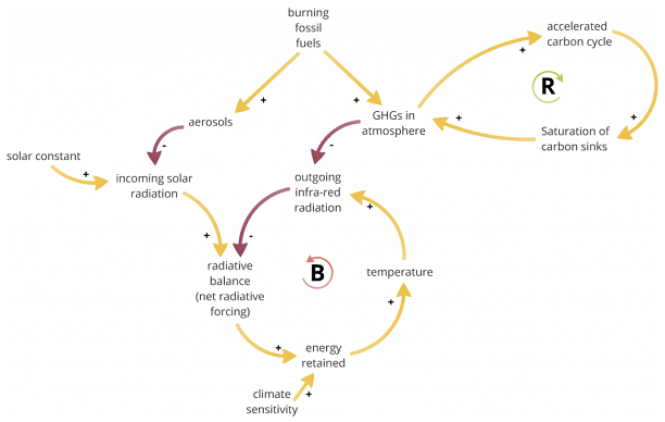
At the start of this series, I argued that Climate Science is inherently a Systems Discipline. To develop that idea, I described two important systems as feedback loops: the earth’s temperature equilibrium loop and economic growth and energy consumption, and then we put these two systems together. 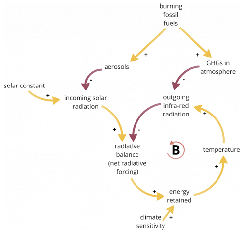The basic climate system now looks like this (leaving out, for now, the dynamics that drive economic development and energy use): The basic planetary energy balancing loop, with the burning of fossil fuels forcing the temperature to change Recall that the balancing loop (marked with a ‘B’) ensures that for each change to the input forcings (in this case greenhouse gases and aerosols in the atmosphere), the earth system will settle down to a new equilibrium point: a temperature at which the incoming and outgoing energy flows are balanced again. Each time we increase the concentration of greenhouse gases in the atmosphere, we can expect the earth to warm, slowly, until it reaches this new equilibrium. The economy-energy system (not shown above) is ensuring that we keep on adding more greenhouse gases, so we’re continually pushing the system further and further out of balance. That means we’re continually increasing the eventual temperature rise that the earth will experience before it reaches a new equilibrium. Meanwhile, the aerosols provide a slight cooling effect, but they wash out of the atmosphere fairly quickly, so their overall concentration isn’t rising much. Carbon dioxide does not wash out quickly – it can remain in the atmosphere for thousands of years. Hence the warming effect dominates. Now, if that was the whole picture, climate change would be very predictable, using basic thermodynamic principles. Unfortunately, there are other feedback loops that we haven’t considered yet. 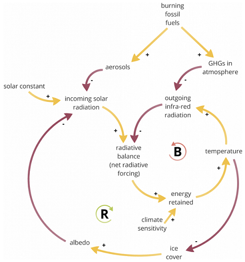Here’s one: The basic climate system with the ice albedo feedback As the temperature rises, the ice sheets start to melt and shrink. These include the Arctic sea ice, glaciers on Greenland and the Antarctic, and mountain glaciers across the world. When sea ice melts, it leaves more sea exposed, which is much darker than the ice. When land ice melts, it uncovers rocks, soils, and (eventually) plants, all of which are also darker than ice. Because of this, loss of ice leads to a lower albedo for the planet. A lower albedo means less of the incoming sunlight is reflected straight back into space, so more reaches the surface. In other words, less albedo means more incoming solar radiation. And, as we already know, this leads to more energy retained and more warming. In other words, it is a re-inforcing feedback loop. As a quick check, we can use the rule of thumb that reinforcing loops have an even number of ‘-’ links. 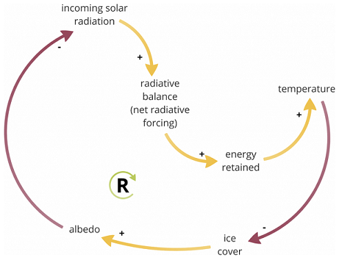Trace the path of this loop to check: Ice albedo feedback loop on its own Because this is a reinforcing loop, it can modify the behaviour of the basic energy balancing loop. If a warming process starts, this loop can accelerate it, and cause more warming than we’d expect from just the main balancing loop. In extreme cases, a reinforcing loop can completely destabilize a system that is normally dominated by balancing loops. However, all reinforcing loops also must have limits (remember: nothing can grow forever). In this case, there is clearly a limit once all the ice sheets on the planet have melted. The loop can no longer function at that point. 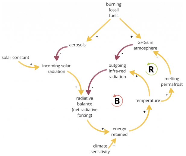Here’s another reinforcing loop: Climate system with permafrost feedback In this loop, as the temperature rises, it melts the permafrost across Northern Canada and Russia. This releases the methane from the frozen soils. Methane is a greenhouse gas, so this loop also accelerates the warming. Again, it’s a re-inforcing loop, and again, there’s a limit: the loop must stop once all the permafrost has melted. Here’s another: Climate system with carbon sinks feedback This loop occurs because the more greenhouse gases we put into the atmosphere, the more work the carbon sinks have to do. Carbon sinks include the ocean and soils – they slowly remove carbon dioxide from the atmosphere. But the more carbon they have to absorb, the less effective they are at taking more. There’s an additional effect for the ocean, because a warmer ocean is less able to absorb CO2. Some model studies even suggest that after a few degrees of warming, the ocean might stop being a carbon sink and start being a source. So, put that altogether and we have three re-inforcing loops working to destabilize the main energy balance loop. 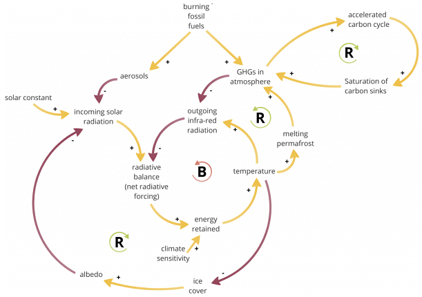The main loop tends to limit the amount of warming we might expect, and the reinforcing loops all tend to increase it: All three reinforcing loops working together Remember, all three re-inforcing loops might operate at once. More likely, each will kick in at different times as the planet warms. Predicting when that might occur is hard, as is calculating the likely size of the effect. We can calculate absolute limits to each of these reinforcing loops, but there are likely to be other reasons why the loop stops working before reaching these absolute limits. One of the goals of climate modelling is to capture these kinds of feedbacks in a computational model, to attempt to quantify the effects, so that we can understand them better. We can use both basic physics and empirical observations to put numbers on each of the relationships in the diagram, and we can experiment with the model to test how sensitive it is to different kinds of perturbation, especially in areas where it’s hard to be sure about the numbers. However, there’s also the possibility that we missed some important feedback loops. In the model above, we have missed an important one, to do with clouds. We’ll meet that in the next post… ABOUT THE AUTHOR Steve M. Easterbrook is a professor of Computer Science at the University of Toronto. Professor Easterbrook's research is focused on software engineering for climate system modeling, and the following is a list of recent publications: Engineering the Software for Understanding Climate Change, Steve M. Easterbrook and Timothy C. Johns, IEEE Computing in Science and Engineering, November 2009. Climate Change: A Software Grand Challenge, Steve M. Easterbrook, Serendipity, 24 August 2010. Guest Editors’ Introduction: Climate Change - Science and Software, S. M. Easterbrook, P. N. Edwards,V. Balaji, R. Budich, IEEE Software, 2011 Why Systems Thinking?, Steve M. Easterbrook, Serendipity, 20 August 2013. The Climate as a System, Part 1: The Central Equilibrium Loop, Steve M. Easterbrook, Serendipity, 22 August 2013. The Climate as a System, Part 2: Energy Consumption, Steve M. Easterbrook, Serendipity, 26 August 2013. The Climate as a System, Part 3: Greenhouse Gases, Steve M. Easterbrook, Serendipity, 27 August 2013. The Climate as a System, Part 4: Earth System Feedbacks, Steve M. Easterbrook, Serendipity, 2 September 2013. The Climate as a System, Part 5: Clouds, Steve M. Easterbrook, Serendipity, 3 September 2013. What Does the New IPCC Report Say About Climate Change?, Steve M. Easterbrook, Serendipity, 8 October 2013. Systems Thinking for Global Problems, Steve M. Easterbrook, Graduate Course Outline, University of Toronto, 2 December 2013. Climate Model vs. Satellite Data, Steve Easterbrook, Serendipity, 14 February 2014. For more information about this author, see his UT Webpage and his Serendipity Blog. |Back to Title| Page 1      Page 2      Page 3      Page 4      Page 5      Page 6      Page 7      Page 8      Page 9 Supplement 1      Supplement 2      Supplement 3      Supplement 4      Supplement 5      Supplement 6 PelicanWeb Home Page